How well can an SVM deal with noise and small samples?
2019-03-21
What I do at my job is called "Multi Voxel Pattern Analysis" (MVPA). It involves applying classification algorithms to functional MRI (fMRI) data, i.e. recorded brain-activity, to predict some parameter or a behavior. The classification algorithm of choice in most studies is the Support Vector Machine (SVM). The reason for this is that commonly we only have small samples (usually ) while the number of features tends to be large (all voxels within multiple volumes, which sums up to ~120000 and more potential features) and SVMs are supposedly good at dealing with small samples and large numbers of features. The accuracies we reach are pretty low most of the time. High enough to yield significant p-values, but not in a useful range to do any predictions. Also fMRI images are quite noisy and a lot of times a positive result becomes insignificant when evaluating it with previously unseen data. This generally made me a little suspicious as to how well an SVM can deal with these difficulties.
Therefore I decided to investigate this a little bit. I generated artificial data using different sample sizes, numbers of features, noise levels and two different decision functions (a linear one, and a circle function). I applied an SVM with a linear and a gaussian kernel to the data, and tested different values for the C and parameters. The source code can be downloaded here
To run it you will have to install a few things first:
pip install click datasheet scipy seaborn scikit-learn toolz cytoolz tqdm
subsequently you can then run the script with python sample_effects.py and
python cl_comparrison.py which will then create an output folder in which you
will find an index.html Depending on your CPU you might want to open the
scripts and adjust the n_jobs variable. The scripts will run a couple of hours.
The file commons.py contains code that is used by both scripts.
Data generation.
For all datasets, the features were drawn from a normal distribution with a mean of 0 and a standard deviation of 1. How the labels were generated depends on the dataset:
- linear: random weights were drawn from the same normal distribution like the features. The labels were then generated by taking the dot product of the feature-vectors and the weights and checking whether it was greater or equal to 0.
- circle: the mathematical formula to check whether a point lies within a circle is where is the offset of the circle center from the origin and is the radius. For one dataset I used and for one I drew from the normal distribution. The radius was chosen by taking the median of the distance of all points from the circle center. This leads to a clean 50/50 split among both classes.
I then applied noise to the features by drawing new features from the normal distribution, and computed the corrupted features by: where are the noise free feats, and is the noise ratio. Subsequently, all features were divided by their standard deviation.
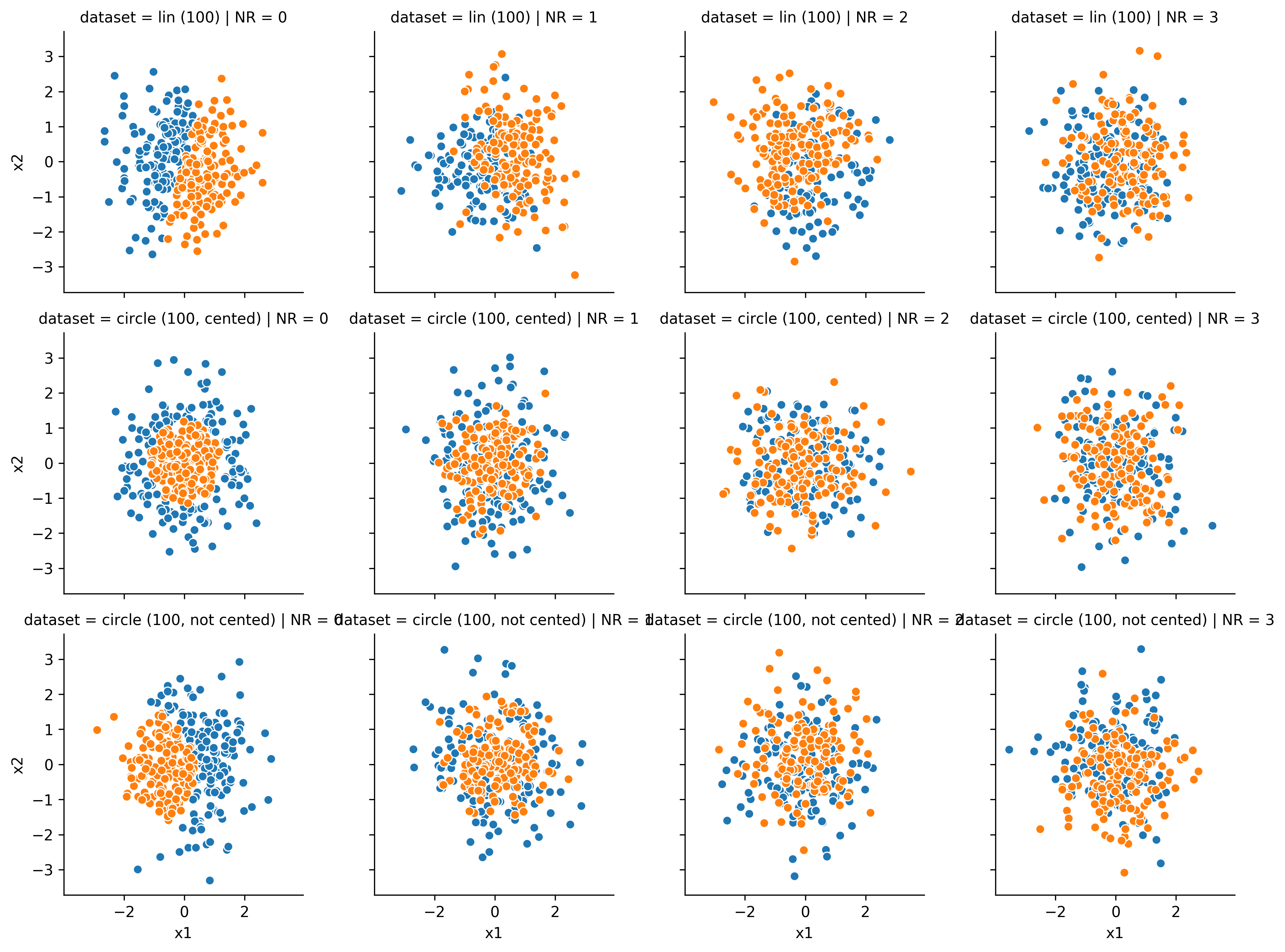
Here are a few examples of how the datasets look in 2D (the NR changes along the columns, and the dataset along the rows):
For each NR, I estimated the "True Information Level" (TIL) by applying the decision function with the chosen parameters to the noisy data, and using the resulting classification accuracy. The following table contains the TILs for the linear dataset. The 2nd number in the cell gives the 95% confidence interval from the 49 repetitions.
| dims | 10 | 30 | 100 | 200 | 1000 |
|---|---|---|---|---|---|
| NR | |||||
| 0 | 1.000+-0.000 | 1.000+-0.000 | 1.000+-0.000 | 1.000+-0.000 | 1.000+-0.000 |
| 1 | 0.752+-0.009 | 0.750+-0.009 | 0.748+-0.010 | 0.749+-0.007 | 0.756+-0.009 |
| 2 | 0.647+-0.009 | 0.652+-0.009 | 0.644+-0.010 | 0.645+-0.009 | 0.647+-0.010 |
| 3 | 0.604+-0.009 | 0.599+-0.009 | 0.598+-0.011 | 0.603+-0.010 | 0.599+-0.012 |
as can be seen, without noise the TIL is obviously 1. With a NR of 1 (i.e. 50% noise) the TIL is roughly at 75% and for NR = 2 it drops 65%. Interestingly the TIL is independent of the number of features (dims).
The next table contains the TIL from the centered circle dataset:
| dims | 10 | 30 | 100 | 200 | 1000 |
|---|---|---|---|---|---|
| NR | |||||
| 0 | 1.000+-0.000 | 1.000+-0.000 | 1.000+-0.000 | 1.000+-0.000 | 1.000+-0.000 |
| 1 | 0.659+-0.010 | 0.667+-0.009 | 0.667+-0.010 | 0.676+-0.009 | 0.670+-0.009 |
| 2 | 0.560+-0.010 | 0.559+-0.011 | 0.566+-0.009 | 0.558+-0.011 | 0.560+-0.013 |
| 3 | 0.535+-0.010 | 0.528+-0.010 | 0.525+-0.009 | 0.538+-0.010 | 0.535+-0.010 |
The impact by the noise is way stronger than on the linear dataset. Although this might come surprising at first, an intuition for this effect can be gained by taking a look of the 2D examples. There it becomes pretty hard to draw a correct line by eye at NR = 1 already.
The third dataset lies somewhere in between:
| dims | 10 | 30 | 100 | 200 | 1000 |
|---|---|---|---|---|---|
| NR | |||||
| 0 | 1.000+-0.000 | 1.000+-0.000 | 1.000+-0.000 | 1.000+-0.000 | 1.000+-0.000 |
| 1 | 0.713+-0.011 | 0.722+-0.009 | 0.716+-0.011 | 0.712+-0.008 | 0.724+-0.008 |
| 2 | 0.617+-0.009 | 0.615+-0.011 | 0.615+-0.010 | 0.611+-0.007 | 0.608+-0.009 |
| 3 | 0.580+-0.010 | 0.576+-0.010 | 0.583+-0.009 | 0.577+-0.009 | 0.586+-0.009 |
Most of the time this decision border behaves like a bended line, since half of the circle lies outside of the point cloud. Therefore the performance is somewhere between the other two datasets.
Now that we know how much information actually is in our data, let's take a look at how well the SVMs can actually learn it.
Comparison of SVM kernels
For each dataset I generated 200 observations, 100 for training, and 100 for testing. For the linear SVM I trained and tested every dataset with the following C values [0.0001, 0.001, 0.01, 0.1, 1, 10, 100, 1000, 10000, 100000], for the gaussian SVM I also tested the following values: [0.001, 0.01, 0.1, 1]. For each C value I used the best gamma value, which was chosen by splitting the training set into 80/20 sub sets, training the SVM with the respective C-value, and each value, and then using the best one. Then the performance was evaluated on the 100 element test set.
These are the results from the linear dataset (the noise ratio changes along the columns, and the kernel along the rows. On the x-axis I used the logarithm to base 10 of the C-values, which makes it easier to look at)
Results of the linear dataset
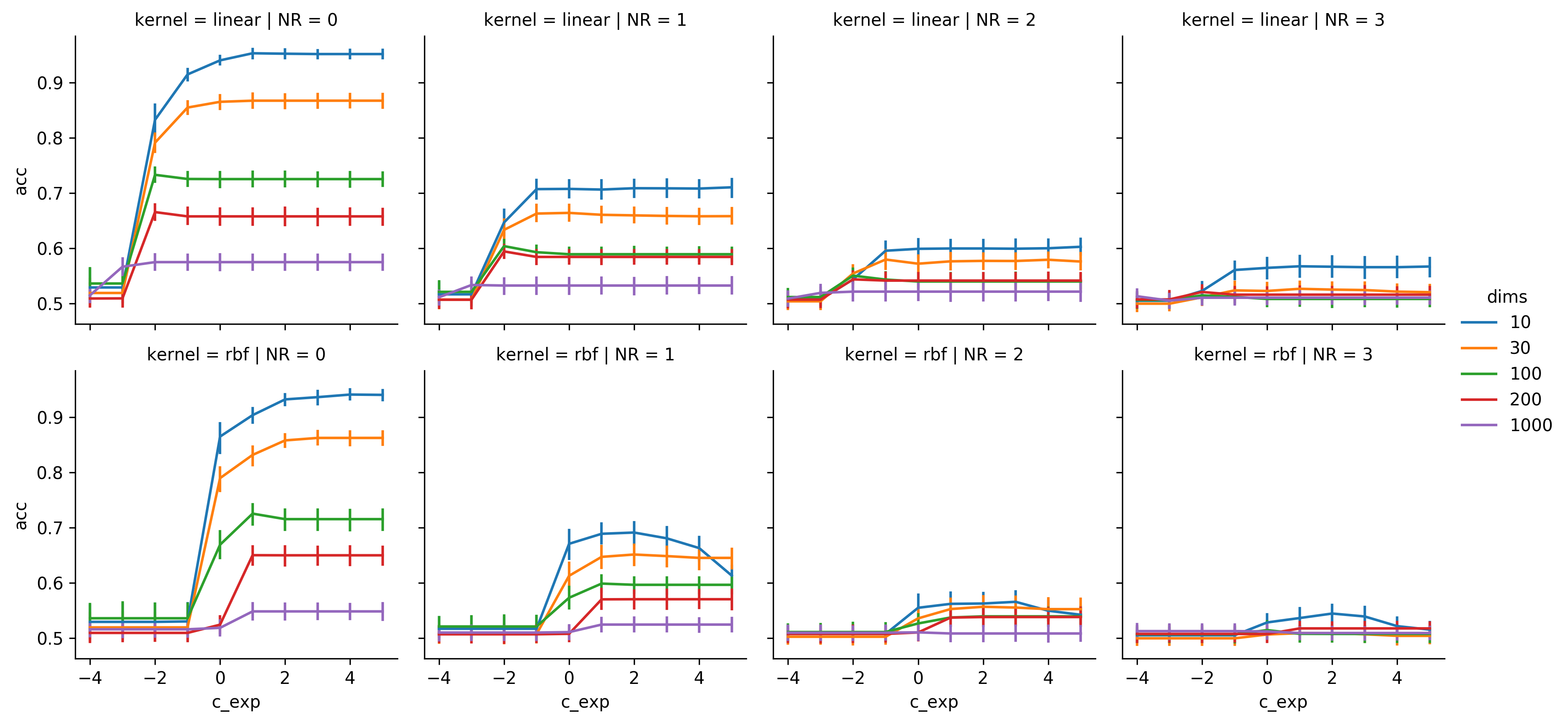
The thing that surprised me the most was that the linear SVM seems to be largely insensitive for the C-Value. As long as it is large enough, there does seem to be an effect. It can be seen that with NR = 0 and for 100 and 200 features C = 0.001 seems to be a little bit better than larger values, but the effect is very weak. For the gaussian kernel, high C-values can reduce the performance quite a bit if there is noise in the data.
Generally for both kernels it can be seen that noise, as well as an increasing number of features both impact the classification accuracy. For dims = 10 both SVMs manage to stay very close to the TIL and perform at most 5% worse. I predicted, that the linear SVM would be quite a bit better than the gaussian SVM on the linear dataset, since the gaussian SVM is a more complex model, but has the same amount of training data. And for NRs of 2 and 3 it indeed has a slight edge, but it is way less than one might have expected.
Results of the circle dataset
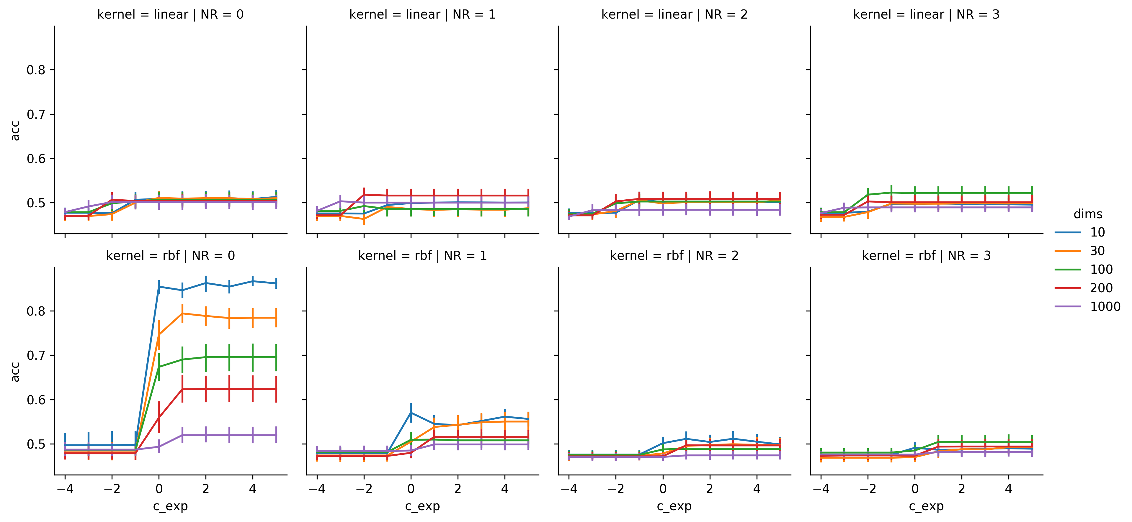
The performance of the linear SVM completely diminished since there is no chance to linearly classify this data. Although performance rises a bit when noise is involved. This would be understandable, if the same data was used for training and testing, but as it was not I'm actually quite surprised to see performances of roughly 53% for NRs of 1 and 3.
The gaussian SVM could perform in this dataset, but even with NR = 0 and dims = 10 the performance is below 90%. I assume, that I should've tested a larger range of values, but since this script takes a long time to compute, and I've already run it over and over for more than a week, I decided that enough was enough. For NR = 1 the performance already gets pretty bad, and only stays above chance level for dims of 10 or 30. This drop is quite a bit larger than in the linear dataset, but the TIL also dropped stronger in this dataset, and the peak of the dims = 10 line actually is only ~7% below the TIL, which is better than in the NR = 0 condition. With NR > 1 classification attempts basically become pointless.
Results of the circle dataset with center offset
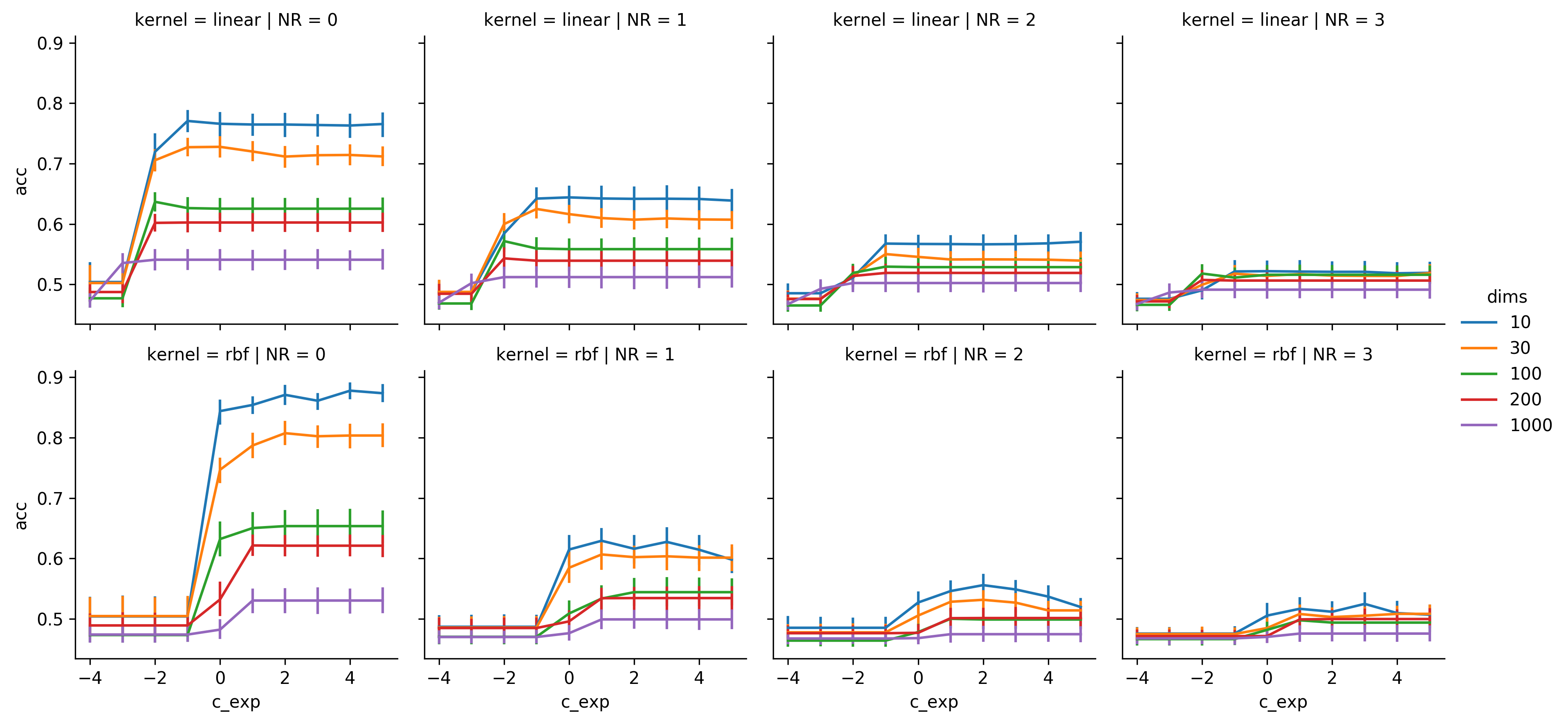
The results from the third dataset are pretty much a mix of the previous ones. The linear SVM reaches mediocre performance, although it's obviously worse than in the linear dataset, and is still outperformed by the gaussian SVM.
Also it can be seen that this dataset is not as noise sensitive as the last one.
So far I would conclude that, given there is enough computation time, it is always better to use a non linear SVM in scenarios like these. The reason for this statement is that both kernels perform essentially identical on the linear data, but the gaussian kernel can also handle non linear data. Generally SVMs are surprisingly good at handling the scenario of (p: number of features, n: number of observations). Even with p = 200 and n = 100 The SVMs generally still reach acceptable classification accuracies for NR = 0. But generally it becomes problematic when noise is involved.
Comparing classifiers
After all of this, I still had the question of how well other classifiers would perform under these circumstances. Therefore I compared the two SVMs to a Random Forrest and a Gradient Boosting classifier. This time I used a training, a test, and an evaluation set. The test set was used to optimize the classifiers parameters, while the evaluation set was used to get the final performance scores of the optimized classifiers for the sake of comparison. For the optimization I tested the following parameters:
- SVM(lin): C: [0.1, 1, 10]
- SVM(rbf):
- C: [0.1, 1, 10]
- : [0.001, 0.01, 0.1, 1, 10, 100]
- RF:
- minimal number of observations per leave: [2, 5, 10, 20]
- number of features per split: []
- GBM:
- learning rate: [0.001, 0.01, 0.1]
- maximum tree depth: [3, 6, 9]
Also I made some changes to the datasets. I used only the centered circle and the linear one, and introduced NR=0.5 while I removed NR=3. Then, I used both datasets twice. First, with a training set size of 100 observations and then with a training set size of 1000 observations. This would allow me to compare the classifiers on ratios of p to n that wouldn't make sense with 100 observations.
These are the results: (this time I didn't include a C-value, therefore it is only one figure with the number of features along the x-Axis, the dataset along the rows and the NR along the cols)
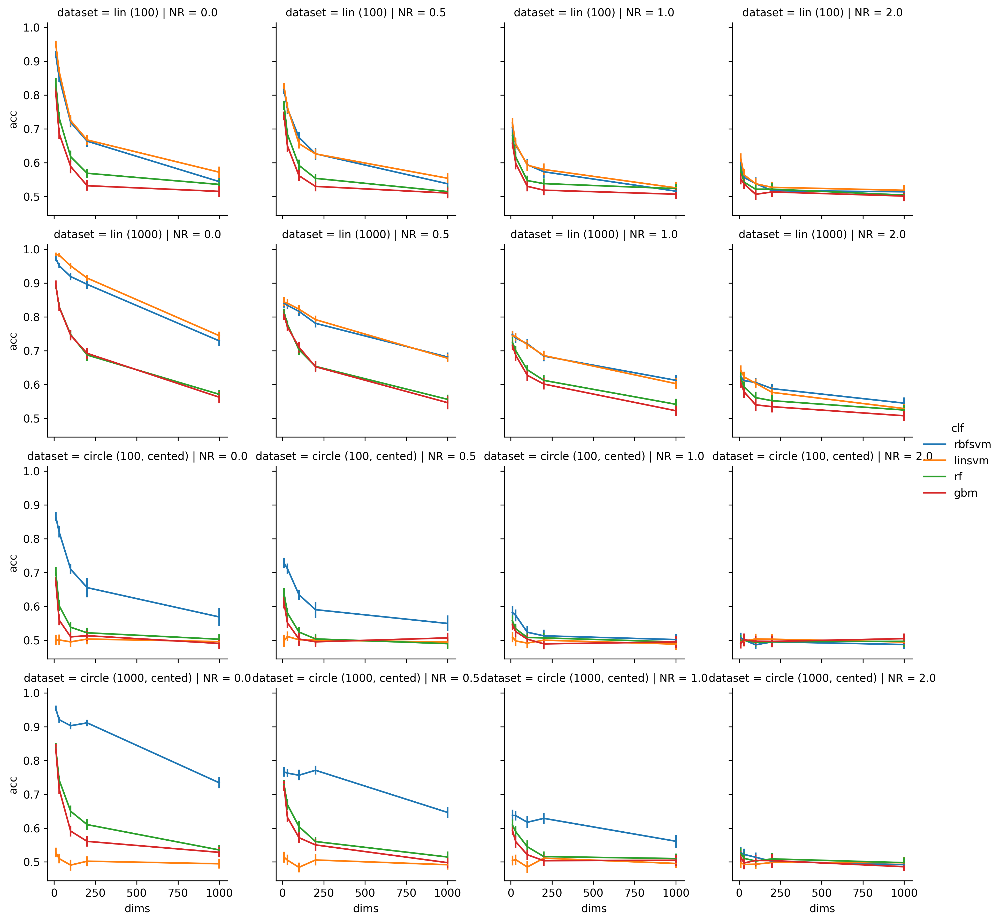
There are 2 clear groups, the first one are the two SVMs, and the second one are the RF and the GBM. Not surprising, given how related these classifiers are. When comparing the plots to the TILs it can be seen, that the SVM basically performs on the level of the TIL if . Good old rules of thumb. It's nice to see evidence for them.
Also it seems that SVM actually are a lot better at dealing with the data than the RF and the GBM. I included the big samples because I expected the second group to surpass the first one there, and I'm quite surprised that it does not. But since the second group is nearly on par with the first one for dim=10 and n=1000 and then falls of exponentially while the SVMs only fall linearly, I assume to have a good chance with these decision tree based models you need . While the SVM still works reasonably wll with , which I would call quite a feature.
None the less, in neuroimaging papers, you commonly see people with less than 100 observations using 1000 and more features, and I suspect that these results might be noise artifacts. Then again, the results often make a lot of sense when looking at the brain areas from which they originated, so maybe the classifiers are actually able to pick up the remaining 2-5% of information.